load balancing
Abstract
There are several algorithm that can be used for a load balancer:
- round robin
- weight round robin: humans tag each server with a weight that dictates how many requests to send to it
- least connections: maintain an accurate understanding of what each server is doing
- peak exponentially weighted moving average: combine techniques from dynamic weighted round robin with techniques from least connections
Past a certain point, web applications outgrow a single server deployment. Companies either want to increase their availability, scalability, or both! To do this, they deploy their application across multiple servers with a load balancer in front to distribute incoming requests. Big companies may need thousands of servers running their web application to handle the load.
In this post we’re going to focus on the ways that a single load balancer might distribute HTTP requests to a set of servers. We’ll start from the bottom and work our way up to modern load balancing algorithms.
Visualising the problem
Let’s start at the beginning: a single load balancer sending requests to a single server. Requests are being sent at a rate of 1 request per second (RPS), and each request reduces in size as the server processes it.
For a lot of websites, this setup works just fine. Modern servers are powerful and can handle a lot of requests. But what happens when they can’t keep up?
Here we see that a rate of 3 RPS causes some requests to get dropped. If a request arrives at the server while another request is being processed, the server will drop it. This will result in an error being shown to the user and is something we want to avoid. We can add another server to our load balancer to fix this.
No more dropped requests! The way our load balancer is behaving here, sending a request to each server in turn, is called “round robin” load balancing. It’s one of the simplest forms of load balancing, and works well when your servers are all equally powerful and your requests are all equally expensive.
When round robin doesn’t cut it
In the real world, it’s rare for servers to be equally powerful and requests to be equally expensive. Even if you use the exact same server hardware, performance may differ. Applications may have to service many different types of requests, and these will likely have different performance characteristics.
Let’s see what happens when we vary request cost. In the following simulation, requests aren’t equally expensive. You’ll be able to see this by some requests taking longer to shrink than others.
While most requests get served successfully, we do drop some. One of the ways we can mitigate this is to have a “request queue.”
Request queues help us deal with uncertainty, but it’s a trade-off. We will drop fewer requests, but at the cost of some requests having a higher latency. If you watch the above simulation long enough, you might notice the requests subtly changing colour. The longer they go without being served, the more their colour will change. You’ll also notice that thanks to the request cost variance, servers start to exhibit an imbalance. Queues will get backed up on servers that get unlucky and have to serve multiple expensive requests in a row. If a queue is full, we will drop the request.
Everything said above applies equally to servers that vary in power. In the next simulation we also vary the power of each server, which is represented visually with a darker shade of grey.
The servers are given a random power value, but odds are some are less powerful than others and quickly start to drop requests. At the same time, the more powerful servers sit idle most of the time. This scenario shows the key weakness of round robin: variance.
Despite its flaws, however, round robin is still the default HTTP load balancing method for nginx.
Improving on round robin
It’s possible to tweak round robin to perform better with variance. There’s an algorithm called called “weighted round robin” which involves getting humans to tag each server with a weight that dictates how many requests to send to it.
In this simulation, we use each server’s known power value as its weight, and we give more powerful servers more requests as we loop through them.
While this handles the variance of server power better than vanilla round robin, we still have request variance to contend with. In practice, getting humans to set the weight by hand falls apart quickly. Boiling server performance down to a single number is hard, and would require careful load testing with real workloads. This is rarely done, so another variant of weighted round robin calculates weights dynamically by using a proxy metric: latency.
It stands to reason that if one server serves requests 3 times faster than another server, it’s probably 3 times faster and should receive 3 times more requests than the other server.
I’ve added text to each server this time that shows the average latency of the last 3 requests served. We then decide whether to send 1, 2, or 3 requests to each server based on the relative differences in the latencies. The result is very similar to the initial weighted round robin simulation, but there’s no need to specify the weight of each server up front. This algorithm will also be able to adapt to changes in server performance over time. This is called “dynamic weighted round robin.”
Let’s see how it handles a complex situation, with high variance in both server power and request cost. The following simulation uses randomised values, so feel free to refresh the page a few times to see it adapt to new variants.
Moving away from round robin
Dynamic weighted round robin seems to account well for variance in both server power and request cost. But what if I told you we could do even better, and with a simpler algorithm?
This is called “least connections” load balancing.
Because the load balancer sits between the server and the user, it can accurately keep track of how many outstanding requests each server has. Then when a new request comes in and it’s time to determine where to send it, it knows which servers have the least work to do and prioritises those.
This algorithm performs extremely well regardless how much variance exists. It cuts through uncertainty by maintaining an accurate understanding of what each server is doing. It also has the benefit of being very simple to implement.
Let’s see this in action in a similarly complex simulation, the same parameters we gave the dynamic weighted round robin algorithm above. Again, these parameters are randomised within given ranges, so refresh the page to see new variants.
While this algorithm is a great balance between simplicity and performance, it’s not immune to dropping requests. However, what you’ll notice is that the only time this algorithm drops requests is when there is literally no more queue space available. It will make sure all available resources are in use, and that makes it a great default choice for most workloads.
Optimizing for latency
Up until now I’ve been avoiding a crucial part of the discussion: what we’re optimising for. Implicitly, I’ve been considering dropped requests to be really bad and seeking to avoid them. This is a nice goal, but it’s not the metric we most want to optimise for in an HTTP load balancer.
What we’re often more concerned about is latency. This is measured in milliseconds from the moment a request is created to the moment it has been served. When we’re discussing latency in this context, it is common to talk about different “percentiles.” For example, the 50th percentile (also called the “median”) is defined as the millisecond value for which 50% of requests are below, and 50% are above.
I ran 3 simulations with identical parameters for 60 seconds and took a variety of measurements every second. Each simulation varied only by the load balancing algorithm used. Let’s compare the medians for each of the 3 simulations:
You might not have expected it, but round robin has the best median latency. If we weren’t looking at any other data points, we’d miss the full story. Let’s take a look at the 95th and 99th percentiles.
Note: there’s no colour difference between the different percentiles for each load balancing algorithm. Higher percentiles will always be higher on the graph.
We see that round robin doesn’t perform well in the higher percentiles. How can it be that round robin has a great median, but bad 95th and 99th percentiles?
In round robin, the state of each server isn’t considered, so you’ll get quite a lot of requests going to servers that are idle. This is how we get the low 50th percentile. On the flip side, we’ll also happily send requests to servers that are overloaded, hence the bad 95th and 99th percentiles.
We can take a look at the full data in histogram form:
I chose the parameters for these simulations to avoid dropping any requests. This guarantees we compare the same number of data points for all 3 algorithms. Let’s run the simulations again but with an increased RPS value, designed to push all of the algorithms past what they can handle. The following is a graph of cumulative requests dropped over time.
Least connections handles overload much better, but the cost of doing that is slightly higher 95th and 99th percentile latencies. Depending on your use-case, this might be a worthwhile trade-off.
One last algorithm
If we really want to optimise for latency, we need an algorithm that takes latency into account. Wouldn’t it be great if we could combine the dynamic weighted round robin algorithm with the least connections algorithm? The latency of weighted round robin and the resilience of least connections.
Turns out we’re not the first people to have this thought. Below is a simulation using an algorithm called “peak exponentially weighted moving average” (or PEWMA). It’s a long and complex name but hang in there, I’ll break down how it works in a moment.
I’ve set specific parameters for this simulation that are guaranteed to exhibit an expected behaviour. If you watch closely, you’ll notice that the algorithm just stops sending requests to the leftmost server after a while. It does this because it figures out that all of the other servers are faster, and there’s no need to send requests to the slowest one. That will just result in requests with a higher latency.
So how does it do this? It combines techniques from dynamic weighted round robin with techniques from least connections, and sprinkles a little bit of its own magic on top.
For each server, the algorithm keeps track of the latency from the last N requests. Instead of using this to calculate an average, it sums the values but with an exponentially decreasing scale factor. This results in a value where the older a latency is, the less it contributes to the sum. Recent requests influence the calculation more than old ones.
That value is then taken and multiplied by the number of open connections to the server and the result is the value we use to choose which server to send the next request to. Lower is better.
So how does it compare? First let’s take a look at the 50th, 95th, and 99th percentiles when compared against the least connections data from earlier.
We see a marked improvement across the board! It’s far more pronounced at the higher percentiles, but consistently present for the median as well. Here we can see the same data in histogram form.
How about dropped requests?
It starts out performing better, but over time performs worse than least connections. This makes sense. PEWMA is opportunistic in that it tries to get the best latency, and this means it may sometimes leave a server less than fully loaded.
I want to add here that PEWMA has a lot of parameters that can be tweaked. The implementation I wrote for this post uses a configuration that seemed to work well for the situations I tested it in, but further tweaking could get you better results vs least connections. This is one of the downsides of PEWMA vs least connections: extra complexity.
Conclusion
I spent a long time on this post. It was difficult to balance realism against ease of understanding, but I feel good about where I landed. I’m hopeful that being able to see how these complex systems behave in practice, in ideal and less-than-ideal scenarios, helps you grow an intuitive understanding of when they would best apply to your workloads.
Obligatory disclaimer: You must always benchmark your own workloads over taking advice from the Internet as gospel. My simulations here ignore some real life constraints (server slow start, network latency), and are set up to display specific properties of each algorithm. They aren’t realistic benchmarks to be taken at face value.
To round this out, I leave you with a version of the simulation that lets you tweak most of the parameters in real time. Have fun!
Abstract
A lot balancer acts as a traffic cop sitting in front of servers and routing clients across all servers with equal load to ensure that no single server has too much load, which can lead to degradation of service or degradation of server’s health. Some LB algorithms used:
- round robin
- weighted round robin
- least connections
- least response time
- ip hash
As the name suggest it has something to do with balancing the load, but here in backend system design architecture load generally refers to traffic or amount of incoming requests 📶
So yeah, going by the name it manages traffic to servers so that they may not get overloaded by traffic ⚖️
Imagine Facebook or Instagram, such a huge giant they are aren’t they now let us assume all of their traffic and backend process is handled by a single server, not even a super computer can do such wonders 😂
So definitely they must have multiple server spread across the globe 🌍 now how to decide which request goes to which server 🤨 And how to make sure that a particular server is not stormed by lot of requests, while other servers sits idle and smile at each other 😆
This is the time when load balancer comes for rescue🦸
It does the job of deciding which request goes to which server, and thus solving the above mentioned problems ✔️
Let’s see this in detail 🕵️
When we talk about a server its not a single server, actually there are lot of server sitting behind load balancer, Load Balancer is a device (hardware) or may be a software (ex: Ngnix)
But when software is available then who will spend money on hardware 💰
So a software load balancer is widely used 🎢
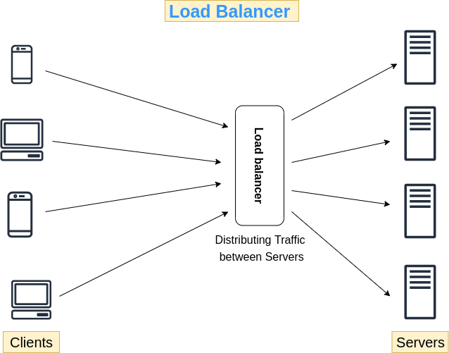
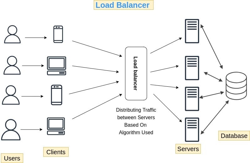
In the above image servers could be web server or application server, and server may further communicate with database etc etc
A load balancer acts as a traffic cop 👮 sitting in front of servers and routing clients across all servers with equal load 📶 This ensures that no single server have too much load which can lead to degradation of service or degradation of server’s health 👨⚕️
- A load balancer divides load uniformly across all servers, in the above scenario every server would receive 25% of the load as there are 4 servers. ♾️
- When client resolves URL into an IP address through DNS Lookup it basically gives the Load Balancer’s IP not server’s IP.
- Requests are measured in QPS (Query per second)
- This Adds extra security 🔐 as servers are not publicly exposed and remains in a private network. If a client tries to directly access servers it cant do so without going through load balancer.
Load balancing Algorithms 🍖
The algorithm in a particular load balancer decide which server will be receiving the next incoming request
The Algorithms are as follow 👇
- Round Robin
- weighted Round Robin
- Least Connections
- Least Response Time
- IP Hash
Lets take a look at all of them in detail 🕵️♂️
Round Robin ⭕
Requests are sequentially sent to 1st, 2nd 3rd,… till last server and then next request is sent back to the first server and this process is continues in a circular manner 🔁

In the above case requests will be sent in this manner:
S1S2S3S4S1S2S3
And So on…
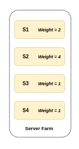
Weighted Round Robin 🏋️
One Drawback in Round Robin is that it assume that all the servers have same computational power and there’s no way we can assign more requests to the one with more power and less request to the one with less power. 🚦
To counter this we assign weights to each server and based on that weight requests are redirected 💪
Least Connections Algo ↔️
Request are sent to server with least number of open connections ⚖️
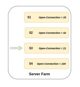
In the above representation at this particular instance S3 has the least number of connections so the next incoming request will be received by server S3 according to Least Connection Algo
Least Response Time Algo 🔭
Request are sent to the server with fewest active connection and lowest average response time ↔️
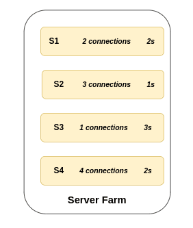
Here the avg response time is calculated by multiplying number of connections and response time
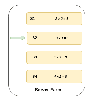
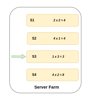
In the first case S2 and S3 both have same avg response time so in that case either of S2 or S3 will receive the request.
But in case 2 S3 has the least avg response time hence it will receive the request
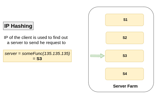
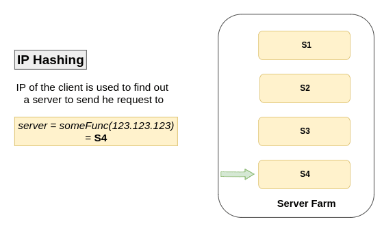
IP Hashing Algo
Here IP of the client is used to determine the server to which request has to be redirected 🥢
An high level explanation would be:
Some logic is written in a function and an IP address is passed to that function, based on that logic which resides inside the function it return the server to which request has to be redirected for that particular IP address 👩🏻🔧
Placement of Load Balancers 🛤️
Based on certain criteria Load balancer can be placed at Layer 4 or Layer 7 in the OSI Model of a product 🧘♂️
An OSI Model consist of 7 layers which are 👇
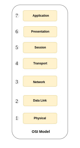
Its Similar to layers in a Cake 🥮 😁
Layer 4 Load Balancers:
The Layer 4 Load balancer are placed on the 4th Layer of OSI model i.e Transport Layer
They don’t have access to data and decision to redirect request to a server is purely done on the basis on data.
Layer 7 Load Balancers:
Layer 7 Load Balancer are placed on Application layer and have access to incoming as well outgoing request and data and decision is made up on its basis, Layer 7 LB is very very much complex :/
At Last an high level architecture of load balancer can be depicted as:
Happy Load Balancing 🚀