the art of solving problems with Monte Carlo simulations
Abstract
The Monte Carlo simulations is fast and easy to implement to find answers to certain problems. Two major applications examples:
- the numerical integration
- how to estimate an option price using the Black-Scholes-Merton model.
This article will explore some examples and applications of Monte Carlo simulations using the go programming language. To keep this article fun and interactive, after each Go code provided, you will find a link to the Go Playground, where you can run it without installing Go on your machine.
Put your adventure helmets on!

Requirements
As stated previously, there is no need to install anything on your computer, you can use the Go Playground. However, if you wish to run the programs locally on your computer (which I recommend), you should download and install Go. If you want to learn the Go Programming Language, check the “Recommended Reading” section at the end of this article, as well as
The Go programming language is deemed to be the most promising programming language today due to its speed and simplicity, and I recommend you to at least get acquainted with it.
Quick Introduction
Generally speaking, Monte Carlo methods (or simulations) consist of a broad class of computational algorithms that rely on repeated random sampling to obtain numerical results. This technique is used throughout areas such as physics, finance, engineering, project management, insurance, and transportation, where a numerical result is needed and the underlying theory is difficult and/or unavailable.
It was invented by John von Neumann, Stanisław Ulam, and Nicholas Metropolis, who were employed on a secret assignment in the Los Alamos National Laboratory, while working on a nuclear weapon project called the Manhattan Project. It was named after a well-known casino town called Monaco, since chance and randomness are core to the modeling approach, similar to a game of roulette.
Here are two excerpts taken from books on Monte Carlo simulations. The first comes from N.T. Thomopoulos’ “Essentials of Monte Carlo Simulation: Statistical Methods for Building Simulation Models”, and the second comes from Paul Glasserman’s “Monte Carlo Methods in Financial Engineering (Stochastic Modelling and Applied Probability)”:
To apply the Monte Carlo method, the analyst constructs a mathematical model that simulates a real system. A large number of random sampling of the model is applied yielding a large number of random samples of output results from the model. […] The method is based on running the model many times as in random sampling. For each sample, random variates are generated on each input variable; computations are run through the model yielding random outcomes on each output variable. Since each input is random, the outcomes are random. In the same way, they generated thousands of such samples and achieved thousands of outcomes for each output variable.
Monte Carlo methods are based on the analogy between probability and volume. The mathematics of measure formalizes the intuitive notion of probability, associating an event with a set of outcomes and defining the probability of the event to be its volume or measure relative to that of a universe of possible outcomes. Monte Carlo uses this identity in reverse, calculating the volume of a set by interpreting the volume as a probability. In the simplest case, this means sampling randomly from a universe of possible outcomes and taking the fraction of random draws that fall in a given set as an estimate of the set’s volume. The law of large numbers ensures that this estimate converges to the correct value as the number of draws increases. The central limit theorem provides information about the likely magnitude of the error in the estimate after a finite number of draws.
If you are new to the subject, keep these ideas in mind to help you understand what follows next.
First Examples
Let’s start our journey with some basic, and even textbook, examples of Monte Carlo simulations. You’re going to notice a pattern when implementing this method. Use it when implementing your simulations.
Estimating π
This is by far the most famous example of Monte Carlo simulations, considered to be the “zeroth example” of the subject. To estimate π, we need to pose the problem in probabilistic terms. We do so by considering a circle of radius r=1 inscribed in a square of side l=2, both centered in the origin of a cartesian coordinate system. This situation is depicted below.
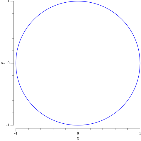
If we were to draw random points in this square, some will fall within the circle and some won’t. But the ratio between points inside the circular region and the total amount of points we draw will be closer and closer to the ratio between the area of the circle and the area of the square as we draw more of these random points.
As you might know, the area of the circular region is A◯=π⋅r2
and the area of the square is A□=(2r)2=4r2. Thus, π=4⋅A◯A□.
As a result, we can estimate π
as π≈4⋅# points inside the circle# points. Remember that, in our case, (x,y) will fall inside the circular region if x2+y2<1.
Now, let’s turn this idea into a Go code.
package main

import (
    "fmt"
    "math"
    "math/rand"
    "time"
)

func main() {
    rand.Seed(time.Now().UTC().UnixNano())

    const points = 1_000_000
    fmt.Printf("Estimating pi with %d point(s).\n\n", points)

    var sucess int
    for i := 0; i < points; i++ {
        x, y := genRandomPoint()

        // Check if point lies within the circular region:
        if x*x+y*y < 1 {
            sucess++
        }
    }

    piApprox := 4.0 * (float64(sucess) / float64(points))
    errorPct := 100.0 * math.Abs(piApprox-math.Pi) / math.Pi

    fmt.Printf("Estimated pi: %9f \n", piApprox)
    fmt.Printf("pi: %9f \n", math.Pi)
    fmt.Printf("Error: %9f\n", errorPct)
}
Run this code in the Go Playground
$ go run euler.go

Estimating e with 1000000 experiment(s).

Expected vale:  2.718631
e:  2.718282
Error:  0.012845%
An astonishing result!
The Birthday Paradox
This is a famous problem in statistics:
In a group of 23 people, the probability of a shared birthday exceeds 50 > %.
That sounds weird at first but, given you’re good enough with math, you can easily prove this statement. However, we are not interested in formal proofs here. That is the whole point of these simulations. The idea is elementary: create a list with n random numbers (in our case n=23) between 0 and 364 representing each person’s birthday, and if (at least) two of them coincide, you increment the success variable. Do it a certain number of times and calculate the probability dividing the number of successes by the total number of simulations.
The corresponding Go code:
package main

import (
    "fmt"
    "math/rand"
    "time"
)

func main() {
    rand.Seed(time.Now().UTC().UnixNano())

    const trials = 1_000_000
    var (
        numPeople = 23
        success   = 0
    )
    for i := 0; i < trials; i++ {
        bdays := genBdayList(numPeople)
        uniques := uniqueSlice(bdays)

        if len(uniques) != numPeople {
            success++
        }
    }
    probability := float64(success) / float64(trials)
    fmt.Printf("The probability of at least 2 persons in a group of %d people sharing a birthday is %.2f\n", errorPct)
}

// randomly sets the game
func setMontyHallGame() (int, int) {
    var (
        montysChoice int
        prizeDoor int
        goat1Door int
        goat2Door int
        newDoor int
    )

    guestDoor := rand.Intn(3)

    areDoorsSelected := false
    for !areDoorsSelected {
        prizeDoor = rand.Intn(3)
        goat1Door = rand.Intn(3)
        goat2Door = rand.Intn(3)
        if prizeDoor != goat1Door && prizeDoor != goat2Door && goat1Door != goat2Door {
            areDoorsSelected = true
        }
    }

    showGoat := false
    for !showGoat {
        montysChoice = rand.Intn(3)
        if montysChoice != prizeDoor && montysChoice != guestDoor {
            showGoat = true
        }
    }

    madeSwitch := false
    for !madeSwitch {
        newDoor = rand.Intn(3)
        if newDoor != guestDoor && newDoor != montysChoice {
            madeSwitch = true
        }
    }
    return newDoor, prizeDoor
}
Run this code in the Go Playground
$ go run monty_hall.go

Estimating the probability of winning by switching doors with 10000000 game(s).

Estimated probability:  0.666447
Theoretical value:  0.666667
Error:  0.032950%
Therefore, contrary to popular belief, it is more advantageous to the guest to switch doors, confirming the theoretical result.
Integration Using Monte Carlo Simulations
Now, let’s see how we can use the Monte Carlo method to find the value of definite integrals of continuous functions in a specified range of its domain. Due to its convergence properties, this method is particularly useful for higher-dimensional integrals.
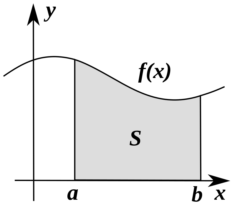
Just as a reminder, if f:[a,b]→R is a continuous function, then the quantity S=∫baf(x)dx, represents the net signed area of the region between the graph of f and the x−axis.
There are some ways to approximate this area, such as Newton-Cotes rules, trapezoidal rule, and Simpson’s rule. However, one clever way to numerically integrate continuous functions is using the formula S≈b−ann∑i=1f(a+(b−a)Ui), where Ui∼U(0,1), i.e. the Ui are uniformly distributed in [0,1] (feel free to try different probability distributions in [0,1] and compare the results).
We are going to use this technique to solve a classic problem. If you are a calculus geek, you might know how difficult it is to calculate the integral S=∫∞−∞e−x2dx.
It involves a trick using Fubini’s theorem and a change from cartesian to polar coordinates. Surprisingly, the result of this integral is √π . Let’s use Monte Carlo integration to evaluate ¯S=∫20−20e−x2dx.
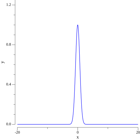
As we can see, f rapidly decreases when moving away from x=0, so the definite integral in [−20,20] seems to be a good approximation.
The corresponding Go code is:
package main

import (
    "fmt"
    "math"
    "math/rand"
    "time"
)

func main() {
    rand.Seed(time.Now().UTC().UnixNano())

    const numPoints = 1_000_000
    fmt.Printf("Estimating the integral of f with %d point(s).\n\n", numPoints)

    integral := monteCarloIntegrator(gaussian, -20.0, 20.0, numPoints)
    fmt.Printf("Approx. integral: %9f \n", integral)
}

// monteCarloIntegrator receives a function to be integrated.
func monteCarloIntegrator(f func(float64) float64, a float64, b float64, n int) float64 {
    var s float64
    for i := 0; i < n; i++ {
        ui := rand.Float64()
        xi := a + (b-a)*ui
        s += f(xi)
    }

    s = ((b - a) / float64(n)) * s
    return s
}

// function to be integrated
func gaussian(x float64) float64 {
    return math.Exp(-x * x)
}
Run this code in the Go Playground
$ go run mc_integration.go

Estimating the integral of f with 1000000 point(s).

Approx. integral:  1.771559
In fact, 1.7715592≈3.138. You should use the Go Playground to experiment with different functions (quadratic, cubic, polynomials in general, or even more complicated functions).
Option Pricing Using the Black-Scholes Model
For the final section of this article, I have something special that draws a lot of attention, the Black-Scholes model. Our goal is to study the evolution of a stock index over time and use the Black-Scholes model to calculate the corresponding option price using Monte Carlo simulations, considered to be a cornerstone for numerical option pricing.
The Black–Scholes, or Black–Scholes–Merton model (Fischer Black, Myron Scholes, and Robert C Merton) , is a mathematical model for the dynamics of a financial market containing derivative investment instruments, giving a theoretical estimate of the price of European-style options and shows that the option has a unique price given the risk of the security and its expected return. This work granted Myron Scholes and Robert C Merton their Nobel Prize in Economics (1997), and has been widely used in algorithmic trading strategies around the world.
The Model
We start with the Black-Scholes-Merton formula (1973) for the pricing of European call options on an underlying (e.g. stocks and indexes) without dividends: C(St,K,t,T,r,σ)=St⋅N(d1)−e−r(T−t)⋅K⋅N(d2)N(d)=1√2π∫d−∞e−12x2dxd1=logStK+(T−t)(r+σ22)σ√T−td2=logStK+(T−t)(r−σ22)σ√T−t.
In the equations above St is the price of the underlying at time t, σ is the constant volatility (standard deviation of returns) of the underlying, K is the strike price of the option, T is the maturity date of the option, r is the risk-free short rate.
The Black-Scholes-Merton (1973) stochastic differential equation is given by dSt=rStdt+σStdZt, where Z(t) is the random component of the model (a Brownian motion). In this model, the risky underlying follows, under risk neutrality, a geometric Brownian motion with a stochastic differential equation (SDE).
We will look at the discretized version of the BSM model (Euler discretization), given by St=St−Δtexp((r−σ22)Δt+σ√Δtzt).
The variable z is a standard normally distributed random variable, 0<Δt<T, a (small enough) time interval. It also holds 0<t≤T with T the final time horizon.
In this simulation we use the values S0=100, K=105, T=1.0, r=0.05, σ=0.2. Let’s see what is the expected option price using these parameters and assuming t=0, then we will run a Monte Carlo simulation to find the option price under the same conditions.
Option Pricing
We are going to use the first set of equations, together with our Monte Carlo integrator, to calculate the option price under the conditions established. The corresponding Go code is:
package main

import (
    "fmt"
    "math"
    "math/rand"
    "time"
)

func main() {
    rand.Seed(time.Now().UTC().UnixNano())

    // Parameters
    S0 := 100.0  // initial value
    K := 105.0   // strike price
    T := 1.0     // maturity
    r := 0.05    //risk free short rate
    sigma := 0.2 //volatility
    numPoints := 250_000

    start := time.Now()
    optionPrice := bsmCallValue(S0, K, T, r, sigma, numPoints)
    duration := time.Since(start)

    fmt.Printf("European Option Value: %.3f\n", optionPrice)
    fmt.Println("Execution time: ", duration)
}

func bsmCallValue(S0, K, T, r, sigma float64, n int) float64 {
    d1 := math.Log(S0/K) + T*(r+0.5*sigma*sigma)/(sigma*math.Sqrt(T))
    d2 := math.Log(S0/K) + T*(r-0.5*sigma*sigma)/(sigma*math.Sqrt(T))

    mciD1 := monteCarloIntegrator(gaussian, -20.0, d1, n)
    mciD2 := monteCarloIntegrator(gaussian, -20.0, d2, n)

    return S0*mciD1 - K*math.Exp(-r*T)*mciD2
}

// MC integrator
func monteCarloIntegrator(f func(float64) float64, a float64, b float64, n int) float64 {
    var s float64
    for i := 0; i < n; i++ {
        ui := rand.Float64()
        xi := a + (b-a)*ui
        s += f(xi)
    }

    s = ((b - a) / float64(n)) * s
    return s
}

// function to be integrated
func gaussian(x float64) float64 {
    return (1 / math.Sqrt(2*math.Pi)) * math.Exp(-0.5*x*x)
}
Run this code in the Go Playground
$ go run option_pricing.go

European Option Value: 7.964
Execution time:  12.171679ms
This is our benchmark value for the Monte Carlo estimator to follow.
The Simulation
package main

import (
    "fmt"
    "math"
    "math/rand"
    "time"
)

func main() {
    rand.Seed(time.Now().UTC().UnixNano())
    start := time.Now()

    // Parameters
    S0 := 100.0          // initial value
    K := 105.0           // strike price
    T := 1.0             // maturity
    r := 0.05            //risk free short rate
    sigma := 0.2         //volatility
    M := 50              // number of time steps
    dt := T / float64(M) //length of time interval
    I := 250_000         // number of paths/simulations
    var S [][]float64

    // Simulating numPaths paths with M time steps
    for i := 1; i < I; i++ {
        var path []float64
        for t := 0; t <= M; t++ {
            if t == 0 {
                path = append(path, S0)
            } else {
                z := rand.NormFloat64()
                St := path[t-1] * math.Exp((r-0.5*(sigma*sigma))*dt+sigma*math.Sqrt(dt)*z)
                path = append(path, St)
            }
        }
        S = append(S, path)
    }

    // Calculating the Monte Carlo estimator
    sumVal := 0.0
    for _, p := range S {
        sumVal += rectifier(p[len(p)-1] - K)
    }
    C0 := math.Exp(-r*T) * sumVal / float64(I)
    duration := time.Since(start)

    fmt.Printf("European Option Value: %.3f\n", C0)
    fmt.Println("Execution time:", duration)
}

// calculates max(x, 0)
func rectifier(x float64) float64 {
    if x >= 0.0 {
        return x
    }
    return 0.0
}
Run this code in the Go Playground
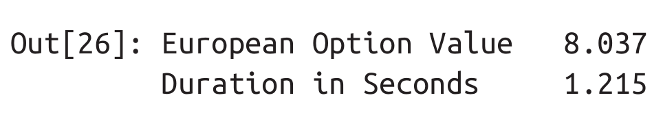
$ go run black_scholes.go

European Option Value: 8.027
Execution time:  430.464289ms
We got a very satisfactory result using the Monte Carlo estimator (remember that the value was 7.964 using the BSM formula and our Monte Carlo integrator).
Let’s compare the results with the same simulation in Python (taken from Yves Hilpisch’s “Python for Finance”):
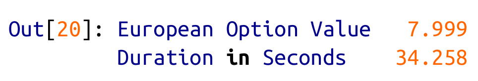
Nearly the same result in a fraction of the time! To be completely fair, when the author uses full Numpy vectorization the results are much better in terms of performance, although we still have a clear winner.
Graphical Analysis
First, let’s plot the simulated index levels (the paths taken during the simulation). The figures below represent the first 10, the first 100, and 250,000 (total number of paths) simulated index levels respectively.
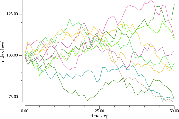
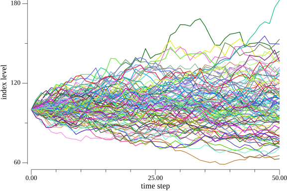
You need to appreciate the fact that each path taken by the index level is an actual possible path, and the option price is calculated by taking every possibility into account.
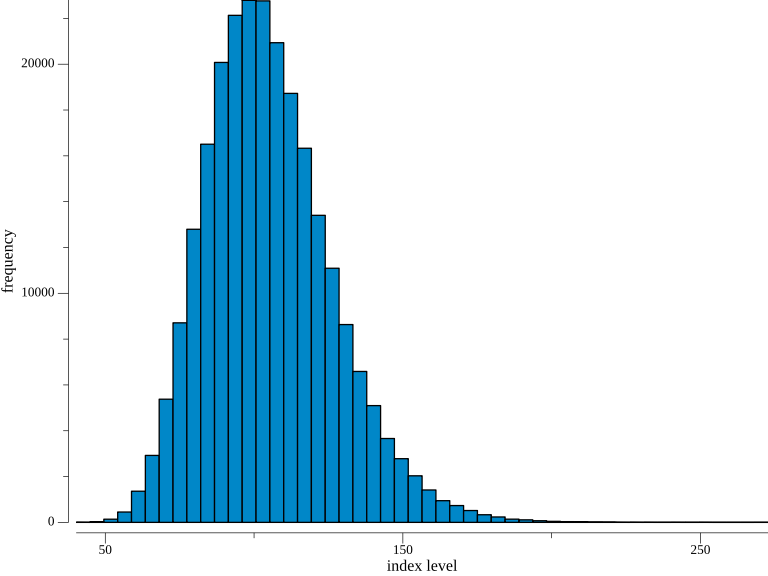
Second, we want to see the frequency of the simulated index levels at the end of the simulation period.
Finally, let’s take a look at the option’s end-of-period (maturity) inner values.
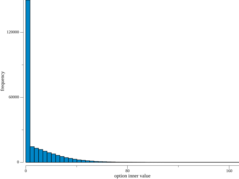
As you can see, the majority of the simulated values are zero, indicating that the European call option expires worthless in these cases.
Conclusion
We have seen basic examples and how one can use the Monte Carlo method to find answers to certain problems. We also have seen two major applications, the numerical integration and how to estimate an option price using the Black-Scholes-Merton model.
By now, you should’ve realized that the Monte Carlo method gives you immense problem-solving powers, even if you’re not very familiar with the underlying theory or even if such a theory doesn’t exist. For instance, see the percolation problem, where no mathematical solution for determining the percolation threshold p has yet been derived.
Now you can successfully apply this technique to your problems and become a practitioner of the art of solving problems using Monte Carlo simulations! Good Luck!